Welcome

The platform is designed to help you plot and visualize some mathematical functions for quantum states in the phase-space framework. Whether you're a student, educator, or professional, FunctionVisualizer helps you understand complex equations and their graphical representations.

Getting Started

From the left hand side you can select the type of function you want to plot.

Modify the different variables of your equation.

Look at your plot from different angles.

Uncertainty Principle

All functions that are plotted must represent physical states. As such, they have to obey the uncertainty principle. The uncertainty principle is an important concept in quantum mechanics. This principle, originally formulated by Heisenberg, states that one cannot know the exact measurement of the position $x$ and momentum $p$ of a particle. There is a limit to the precision expressed through the inequality

\[ \Delta x \Delta p \geq \frac{\hbar}{2} \]

If for example you know the momentum and you try to find the position you do not get the exact value, but only a probability of where that particle might have been at time $t$.

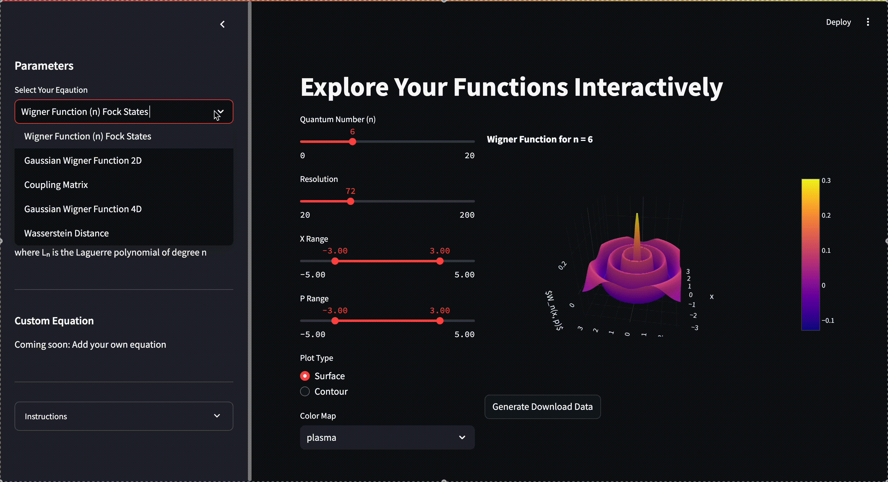
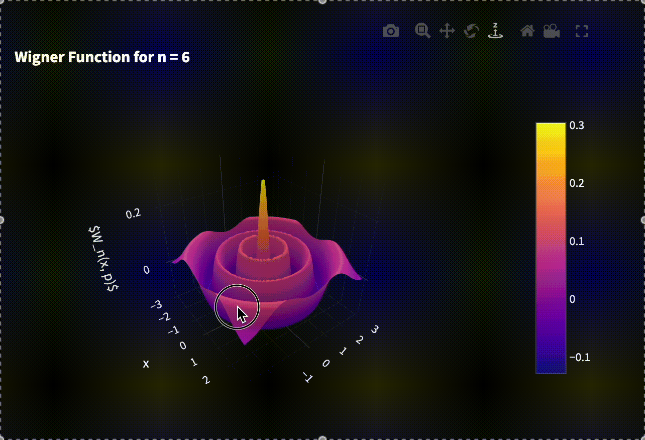
Wigner Function

The Wigner function is a quasi-probability distribution function used in quantum mechanics to represent a quantum state of a system in the phase space. It provides a way to visualize the probability of measuring the position or the momentum of a quantum system, allowing for the analysis of its properties and dynamics. This distribution is not a true distribution as it can become negative, showcasing here a quantum feature of some states. A Fock state is a quantum state which has exactly $n$ photons (or quanta of light). They are represented by the following Wigner function where $L_n(x)$ are the Laguerre polynomials.

\[ W_n(x,p) = \frac{(-1)^n}{\pi}\,e^{-(x^2 + p^2)}\,L_n\bigl(2(x^2 + p^2)\bigr) \]

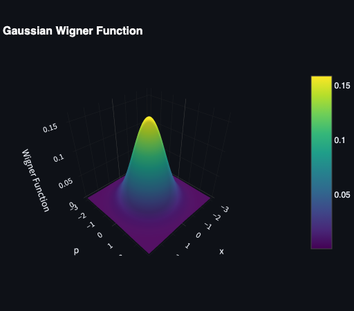
Gaussian Wigner Function 2D

The Gaussian Wigner function is a specific form of the Wigner function that describes a Gaussian state in phase space. It is completely characterized by the first moments (average value of position $\langle x \rangle$ and momentum $\langle p \rangle$) and covariance matrix $\gamma$ whose elements are given by:

\[ \gamma _{ij} = \frac{1}{2}\langle\{\hat{r}_i,\hat{r}_j\}\rangle - \langle{\hat{r}_i}\rangle\langle{\hat{r}_j}\rangle.\]

Here, {.} stand for the anti-commutator and $r$ is a column vector of the position and momentum variables of a particle, that is $r = (x, p)^T$. On this platform, we will only consider states that are centered at the origin such that $\langle{x}\rangle = \langle{p}\rangle = 0$. Therefore, the Gaussian Wigner function is defined as

\[ W(r) = \frac{1}{2\pi\sqrt{\det(\gamma)}}\,e^{-\tfrac12\,r^T\gamma^{-1}r} \]

Note that $\gamma$ must satisfy the uncertainty principle of Heisenberg, but also its improved version from Robertson-Schrödinger, which states that the determinant of the covariance matrix must be greater than or equal to $\frac{\hbar^2}{4}$. This uncertainty principle can also be written as

\[ \gamma \pm \frac{i\hbar\Omega}{2} \geq 0 \quad \text{where} \quad \Omega = \begin{bmatrix}0 & 1\\-1 & 0\end{bmatrix} \]

Note that on this platform, we chose to put $\hbar = 1$ and the commutator of $x$ and $p$ is given by $[x, p] = i.$

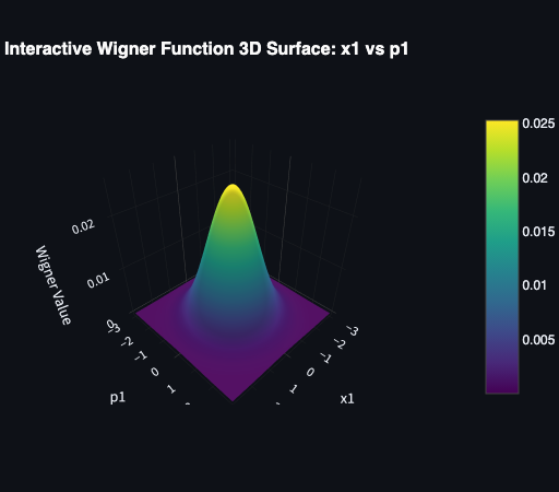
Gaussian Wigner Function 4D

The Gaussian Wigner function in four dimensions extends the concept of the 2D Gaussian Wigner function from 1 particle to 2 particles. It is used to represent more complex quantum states and their interactions. The 4D Gaussian Wigner function is defined similarly to the 2D case, but it describes a two states-system $A$ and $B$, each represented by a $2\times2$ covariance matrix. As such, the global covariance matrix $\gamma$, describing the Gaussian function, is now a $4\times4$ matrix and the vector $r = (x_A, p_A, x_B, p_B)^T$ is 4 dimensional. Still considering states centered at the origin, the Wigner function is given by:

\[ W(r) = \frac{1}{(2\pi)^{2}\sqrt{\det(\gamma)}}\,e^{-\tfrac12\,r^T\gamma^{-1}r} \]

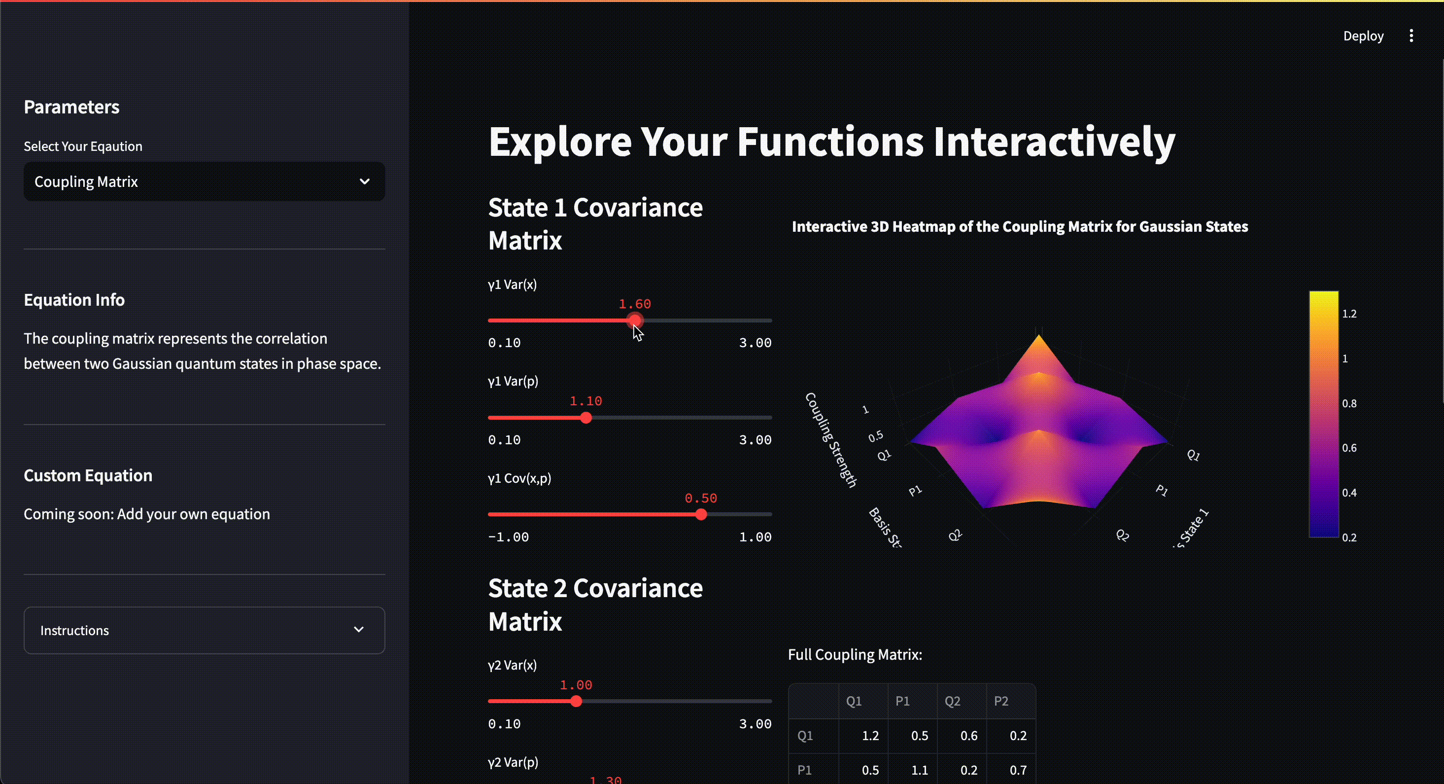
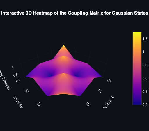
Coupling Matrix

A coupling between two states is a higher dimension system that reduces to the original states when one look at the marginal, but contains some more information in the correlations. When both states are Gaussian, the coupling is Gaussian too and as such, is described by a covariance matrix. The coupling matrix is essential in the calculation of some quantities such as the Wasserstein distance.

Let us assume we have two states represented by covariances matrices $A$ and $B$, each satisfying the uncertainty principle and let us define

\[A^\pm = A \pm \frac{i\Omega}{2}\]

and similarly for $B^\pm$. The coupling matrix is a $4\times4$ matrix that describes the interaction between the two states. It is defined as:

\[ \gamma\Pi = \begin{bmatrix} A & X^T\\ X & B \end{bmatrix} \]

where $X$ can be anything as long as it verifies:

\[X^T A^{-1} X \le B\]

(which is just an expression of the uncertainty principle). With the coupling matrix, we can analyse the possible interactions between the two states and how they influence each other.

The image below shows a 3D plot of a coupling matrix. The $X$ and $Y$ axes represent the basis states, and the $Z$ axis represents the coupling strength between the two states. The color gradient indicates the degree of coupling, with darker colors representing stronger interactions.

Here, the position variable is represented by the letter $Q$ and the momentum by the letter $P$. The first system is described by the covariance matrix $A$ and the second by the covariance matrix $B$.

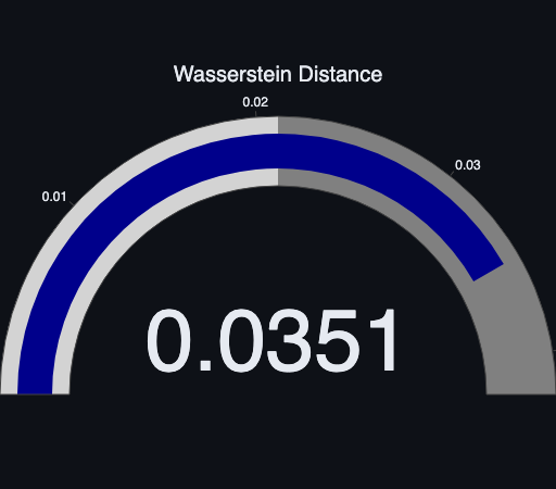
Wasserstein Distance

The Wasserstein distance is a metric used to measure the distance between two probability distributions. In the context of quantum mechanics, it can be used to quantify the differences between quantum states represented by their Wigner functions. The Wasserstein distance is the result of an optimization over all possible couplings between the two states. When both states are Gaussian, the Wasserstein distance is defined as

\[ W(\rho_A, \rho_B)^2 = \frac{1}{2}TrA+\frac{1}{2}TrB-Tr[X_\text{optimal}] \]

where $A$ and $B$ are the covariance matrices of the two states, and $X_\text{optimal}$ is given by:

\[|X| = \sqrt{\sqrt{A^\pm}B^{\mp}\sqrt{A^\pm}}\]

The Wasserstein distance is a powerful tool for comparing quantum states and analyzing their properties. It is particularly useful in quantum information theory and quantum optics. For example, the Wasserstein distance can demonstrate the optimal path between two states $A$ and $B$ where the value of the cost function is at a minimum.

Try it For Yourself

Ready to explore your functions? Click the button below to visit the platform.